mdk

Curvy blues

27 Oct 2007 » permalink

I was looking in the past (and some more) at various solutions for efficient hardware-aided curve rasterization methods. Those ideas mostly focused on using the graphical hardware for accelerating the geometry generation process. But what happens, when we completely skip the geometry generation step? Even more blazing performance and totally resolution-independent rendering. Thanks to some tips by Jon and interesting math discussions I had in the past weeks, I'm glad to present my current thinking.

Quadratic curves

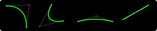
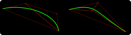
Quadratic curves (second-degree polynomials) consist of a starting point, an end point and one control point. Such curves cannot self-intersect nor inflect. The representation of a quadratic curve is a parabola, a straight line or (a degenerate case) — a point. Quadratic curves are not the most popular ones in modern graphical packages. Cubic types (more about them later) are the basic unit of notation. In example, cairo doesn’t provide direct quadratic API. It’s understandable as any quadratic can be trivially represented in a cubic form. However, since (due to their limited properties) quadratics are usually much faster to process it makes sense to look at them separately. Quadratics are part of the SVG standard and have some interesting uses — including TrueType fonts (which are represented only with 2nd degree curves) and Flash (which uses quadratics as the native curve representation and represents cubics by subdividing them into quadratics). Few examples of quadratic curves:

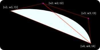
Now, let’s look at how we can hook up the programmable GPU hardware to rasterize quadratics. The first observation is that the three points describing the curve form a triangle and this triangle covers the whole area of the curve. Triangle is the most basicrasterization primitive in modern graphics hardware. Let’s assign two texture coordinates (v and w) for each of the three points. We’re going to use [0.0; 0.5] , [0.0; 1.0] and [1.0; 1.0] for, respectively — the start point, the control point and the end point.

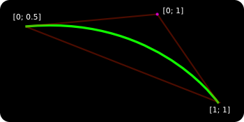
As the triangle is being rendered the hardware will interpolate v and w across the three vertices. For each pixel belonging to the triangle we get a unique, interpolated v and w texture coords pair. And here comes the crucial part — as the actual “texture” for this triangle we use a dynamic fragment program that evaluates the following expression:

If the expression evaluates to true, we pass the pixel. If not, we discard it. What we get is:

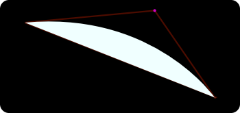
Here is a shader implementation that does this operation. As we see, the rastered picture represents the curve we’re trying to visualize. To be precise, we get the fill for the curve. If we replaced the < sign with = sign we would get the actual stroke (the green line). As we zoom towards the curve, the shader generates more pixels giving a more accurate representation. A true resolution-independent rendering.

I'm going to come back to why this is so fundamentally amazing later on, but now let’s move on to the cubics.

Cubic curves

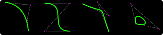
Cubics (third-degree polynomials, the bezier-curves) are a bit more complex. They consist of two arbitrary control points plus start/end points. As a result a cubic can self-intersect, loop, inflect or cusp. Beziers are the thing in vector drawing and most of the data we get to render these days (icons, buttons, UI elements…) are sets of shapes defined by cubic curves.

For blazing-fast rendering of cubics we’re going to use a similar approach that we used for quadratics. Since cubics consist of four points we need more than a single triangle. Actually, depending on the control points set we’re dealing with, we need 2 or 3 triangles. In other words — we need to triangulate the points. In this case (very fixed) triangulation is trivial and essentially we can discover the case we have by doing a few dot products between the vectors of the control points.

Since we’re dealing with a cubic equation, we need three texture coordinates per point (that’s perfectly fine with the OpenGL API). Let’s call those three coords: v, w and t. In our fragment shader (implementation here) we’re going to evaluate the following expression:

And the last hard part — unlike quadratics, for cubics there are no static texture coords to use. We need to calculate them separately for each curve. The method to do that is a subject for a separate article, but it’s enough to say that it’s a fast fixed-time operation that involves few matrix multiplications. Essentially we need to put the control point coordinates in a matrix, move it to power basis and analyze the determinants. Depending on the number of square roots, we have one of the few distinct cubic-cases which further dictate which v, w, t coords to use. Those computations could be put in hardware-accelerated matrix pipeline but I haven’t found that to be critical enough to do so.

In the end we end up with:

Using this technique we can render any cubic at any resolution in a fixed time.

Practical results

Two following screenshots (click for bigger versions) show sample renderings (a font glyph and a mono-project logo) obtained using this method. Shapes consist of roughly 30 cubics/lines. The first figure represents the inner-mesh hardware-accelerated triangulation. The second one — a rendering of the curve data. By combining the two we end up with a final mask for the shape. This method works for any polygon including complex self-intersecting concave/convex shapes.

Why it’s cool

• Traditional approaches to curve rasterization usually require recursive subdividing of the curve towards a certain level of line-approximation or reaching a pixel-precision. The complexity/processing time grows exponentially and the result might be not correct. With the approach presented above we achieve high quality by keeping the mathematically-correct (not compromised) information about the curve till the very last step — the rasterization . The precision of the final image (output) is only limited by the resolution of the display system, not the implementation. The complexity of the algorithm is linear and the processing time is only constrained by the pixel fill rate of the GPU board (that value approaching hundreds of millions for modern equipment).
• From my experiments, attaching the (presented) fragment shaders to the triangle rasterization process has no any impact on the performance. In other words, it seems that on modern hardware rendering a solid-filled triangle is equally fast as rendering a triangle with a simple shader.
• As we’re not generating/storing any extra geometry data and just using two (max three) triangles per curve, the memory requirements are minimal — even for extremally complex shapes.
• By using some additional extensions (such as a compiled vertex array) after the initial pre-calculation step we can completely move the geometry data to the GPU unit and render by just invoking display lists. In this case the expose events theoretically come cost-free for the CPU.

Smart curve rasterization is the first step towards efficient drawing API implementation. By combining the solution with additional dynamical GPU-programmable pipeline elements (gradients, triangulation, anti-aliasing, multi-sample rendering) we can achieve blazing-fast vector-based drawing tool. This is my current approach towards building a new OpenGL-based cairo backend. World domination follows. Obviously.

Update: for better math overview check this article by Loop & Blinn. It’s a good starting point even though it’s not complete and has certain mistakes (check comments).